RBF Nodes
RBF Nodes is a node-based Radial Basis Function (RBF) solver for Blender. It allows multiple input values to drive multiple output targets, overcoming the limitations of Blender’s standard driver system, which typically supports only a single output per driver.
Radial Basis Functions are used to interpolate or approximate values based on a defined set of sample points. They are particularly useful when conventional driver setups fall short, especially in cases involving complex relationships between multiple inputs and outputs. While Blender drivers can combine inputs, they output only a single value. RBFs, by contrast, can compute multiple outputs from multiple inputs.
RBF Nodes is especially well suited for rigging, deformation, and animation control, but it is not limited to these uses. It supports integration with objects, armatures, materials, and Geometry Nodes, making it a flexible solution across a variety of workflows.
1. Introduction
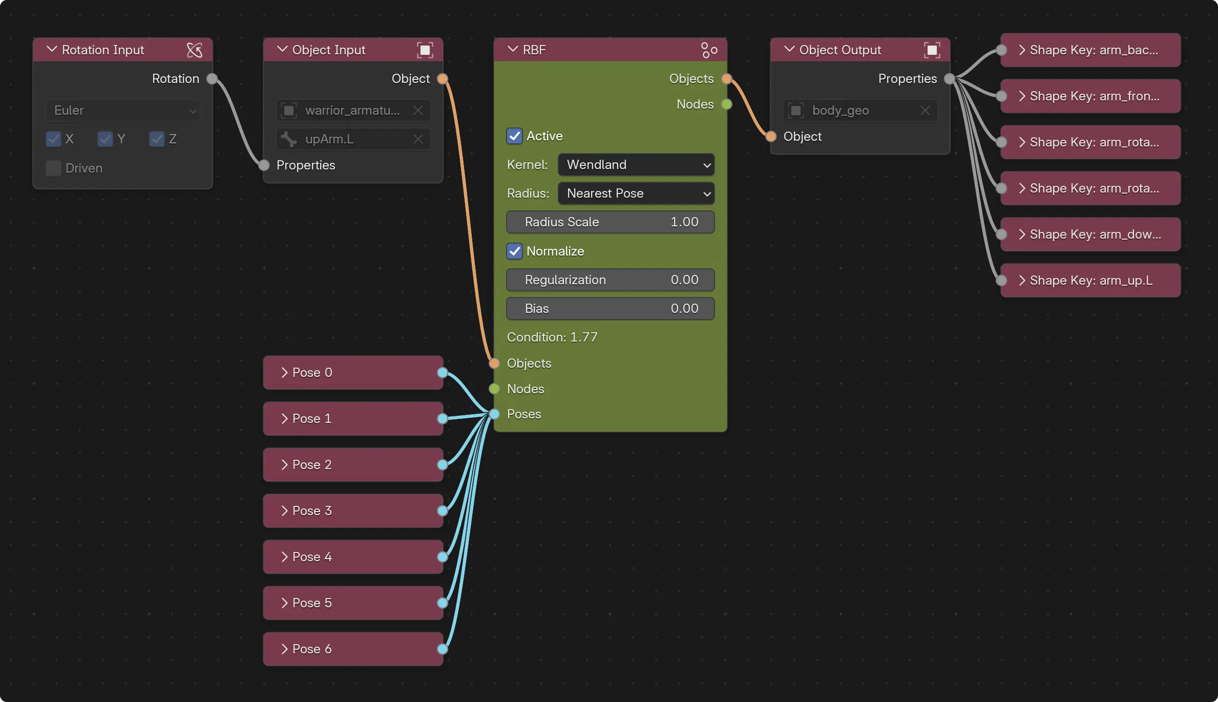
1.1 Overview
RBF Nodes introduces Radial Basis Function interpolation into Blender via a custom node tree. Rather than being limited to single-output drivers, RBF Nodes allows multiple input channels (e.g., transforms, custom properties, shader parameters) to influence multiple output targets simultaneously.
1.2 Key Features
- Multi-Dimensional Interpolation: Drive several outputs from multiple inputs in one solver without the need of complex expressions or scripts.
- Pose-Based Sampling: Capture sample poses that define input/output states for interpolation.
- Broad Compatibility: Works with objects, armatures, Geometry Nodes, and shader properties.
- Performance-Optimised: Precomputes RBF weights to minimise per-frame overhead.
- Scene Linking (NEW in v2.0): Link RBF trees across scenes for modular rigs.
- Constraint & Driver Support (NEW in v2.0): Includes transforms which are constrained or driven.
- Rotation Smoothing (NEW in v2.0): Filter jitter in quaternion or constraint-driven rotations.
1.3 Use Cases
- Facial rig interpolation based on controller positions.
- Procedural animation blends in Geometry Nodes setups.
- Shader parameter blending driven by object transforms.
- Complex rig behaviors without helper bones or custom scripts.
2. Release Notes
Version 4 of RBF Nodes introduces major changes to improve flexibility, stability, and compatibility with Blender’s scene linking system. Below is an overview of the most significant updates and modifications.
2.1 Compatibility
-
Existing RBF setups from earlier versions are not compatible with this version. See Version Compatibility .
-
Object assignments in Object Input and Output nodes are no longer stored as data block pointers. Instead, only object or bone names are stored. This change is required to support scene linking and prevents automatic updates when objects are renamed.
2.2 RBF Core Improvements
- The internal RBF solver has been revisited for improved interpolation stability.
- Wendland is now the default interpolation kernel, which features a smooth fall-off and reaches zero beyond its radius.
- The Gaussian 2 interpolation kernel has been removed. The former Gaussian 1 kernel is now simply called Gaussian.
- The behavior of Radius has been unified across all interpolation kernels. All kernels now exhibit wider influence as the Radius increases. These changes affect existing setups directly.
2.3 Scene Linking Support
- Full support for linked RBF setups in other scenes has been added.
- Library Overrides are required for evaluation of linked setups. See Scene Linking and Library Overrides for details.
2.4 New Features
- Support for indirect transformations from constraints and drivers.
- New option to enable/disable Normalization of input values.
- Added Regularization property to improve pose stability.
- Added Bias value to refine how interpolation balances between samples.
- Poses now store the current frame, which can be recalled optionally for more accurate evaluation.
- New option to disable poses.
- It's now possible to add input or output properties to existing poses.
- Added Export and Import operators for external editing and rebuilding.
- When switching from automatic to manual shape key or custom property selection, the name is preserved to avoid referencing errors.
2.5 Utilities and Operators
New operators in the Sidebar:
- Update Poses for adding new properties to existing poses.
- View Pose and RBF Data in the console for inspection.
- Rename object and property names stored in poses.
- Export and Import for editing and rebuilding.
3. Installation and Setup
RBF Nodes is implemented as an Extension for Blender 4.2 and later.
3.1 Installing the Extension
- Download RBFNodes.zip.
- Drag-and-drop the archive into the Blender window.
- Choose a User Repository from the dropw-down menu.
- Make sure the Enable Add-on option is checked.
3.2 Accessing the Node Editor
- Change any area’s editor type (upper-left dropdown) to RBF Nodes Editor.
4. Version Compatibility
Existing RBF setups from earlier versions are not compatible with this version, mainly because of two significant changes:
-
Pose Data Storage
The internal storage of pose data has been revised. This change affects how pose values are managed by the solver, making earlier setups incompatible with the current version. -
Scene Linking Support Since version 2.0, RBF Nodes supports scene linking. As a consequence, the Object Input and Object Output nodes now store associated object references differently than in previous versions. Only the name of the driver object or bone is stored, not a direct reference to the object’s data block. Storing a pointer would interfere with linking the RBF setup into another scene. Because only the name is stored, it does not reflect any name changes that might occur after assigning the object to the node.
Therefore, existing setups created with earlier versions must be rebuilt in order to work with this version.
When opening a scene with an outdated setup:
- A warning will inform about the incompatibility.
RBF setups created with previous versions may behave differently in this updated version. This is due to internal improvements to the solver algorithm, which affect how poses are blended and activated. While these changes increase accuracy and flexibility, it’s recommended to review and adjust older setups as needed to ensure consistent results.
5. Interface Overview
The RBF Nodes editor is the dedicated environment for building pose-based interpolation trees. This single access point makes it possible to make the RBF setup selection and object independent.
5.1 Node Tree
The node tree contains all nodes and links which relate to an RBF setup. The intention is to have each RBF setup in its own tree, but it’s also possible to have multiple setups in one tree. Since neither the node tree nor any of the nodes has a direct relation to any other data in the scene it’s up to the user to decide how to manage multiple RBF setups.
5.2 Sidebar and UI Elements
With the RBF Nodes editor active, press N to open the Sidebar.
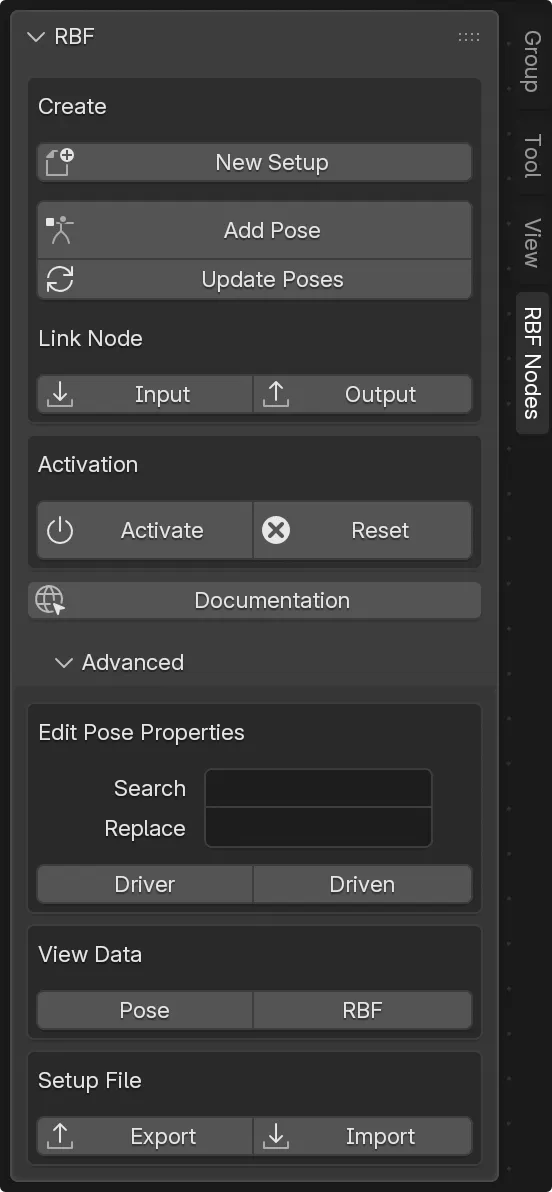
New Setup
Generates a base node tree as a starting point for the setup.
It’s also possible to create a new node tree by using the standard editor buttons for creating a new tree or duplicating the existing, and then adding the required nodes manually.
Add Pose
Captures current driver and driven properties as a pose. The pose is represented as a node which is connected to the
Poses
socket of the
RBF
node.
Update Poses
Matches all existing poses to the current inputs and outputs, so that an input or output can still be added once poses exist. See Changing Inputs and Outputs Later.
Link Node: Input
Create a new input node from the current node graph selection in the
Shader Editor
or
Geometry Node Editor.
Link Node: Output
Create a new output node from the current node graph selection in the
Shader Editor
or
Geometry Node Editor.
Export and Import
Write the node tree to a json file next to the scene, and rebuild it from one. See Export and Import.
Activate
Performs interpolation precomputation and enables runtime evaluation. The background color of the RBF node will turn green if the activation was successful, red in case of an error.
Reset
Removes driver links and deactivates the solver.
More options are available in the
Advanced Settings
subpanel.
5.3 Adding and Connecting Nodes
Add Node
Shift + A → Input / Output / RBF
Sockets
Sockets are color-coded:
| Socket Type | Color | Input Links | Output Links |
|---|---|---|---|
| Object | Orange | Multi | Multi |
| Property | Grey | Single | Multi |
| Nodes | Green | Multi | Multi |
| Poses | Blue | Multi | Single |
All node sockets support multiple connections. The only exception are driven property sockets and pose output sockets.
For example, if multiple properties of an object are being used to drive the setup, such as translation, rotation and scale, each property node connects to the Properties input socket of the Object Input node.
When multiple objects act as drivers, each with their own properties, all related Object Input nodes are connected to the Objects input socket of the RBF node. The same structure applies to drivers based on Shader or Geometry Nodes; these are connected via their respective Node Input nodes to the Nodes input socket of the RBF node.
The output side follows the same modular approach. The Objects and Nodes output sockets of the RBF node can each connect to one or more Object Output nodes or Node Output nodes. Each Object Output node connects to its relevant property nodes through the Properties output socket.
This structure allows multiple input sources to converge into the RBF solver node and enables the results to be distributed across multiple outputs.
5.4 Fake User and Data Persistence
Due to the missing data relationships between the RBF nodes and other Blender data blocks each RBF node tree is set to Fake User to avoid unwanted data removal as long as the RBF solver has not been activated.
6. Workflow
A typical RBF Nodes workflow involves:
- Setup creation
- Defining the driver object/s and properties
- Defining the driven objects/s and properties
- Setting poses
- Solver activation
The following steps outline the process.
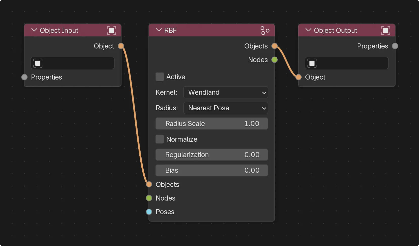
6.1 Creating a New Setup
- In the RBF Nodes editor, open the Sidebar by pressing N (if not already open).
- Click New Setup.
-
A new a base node tree is created with:
- One
RBF Node
in the center
- One Input Object node on the left
- One Output Object node on the right
6.2 Defining Input Properties
- Select the Object Input node.
- Assign the driving object or bone (this is name-based and doesn’t update upon renaming).
- Add one or more property-specific nodes by pressing Shift + A → Input or from the menu choose Add → Input
- Connect each property node’s output to the Properties socket of the Object Input node.
- Adjust the properties of each Property node, if applicable.
- For shader- or Geometry Node-driver outputs, associate the according node via Link Output Node in the RBF Nodes editor and select the driving property on the node.
6.3 Defining Output Properties
- Select the Object Output node.
- Assign the driven object or bone name.
- Add one or more property-specific nodes by pressing Shift + A → Output or from the menu choose Add → Output
- Connect the Properties socket of the Object Output node to each property node’s input socket.
- For shader- or Geometry Node-driven outputs, associate the according node via Link Output Node in the RBF Nodes editor and select the driven property on the node.
6.4 Capturing and Managing Poses
- Set the properties used as input drivers to assume the rest state of the pose.
- Set the properties used as driven outputs to assume the rest state of the pose.
- Click Add Pose in the Sidebar.
- A Pose node appears and connects to the RBF node’s Poses input.
- In preparation for the next pose set the properties used as input drivers accordingly.
- Set the properties used as driven outputs to reflect the next pose.
- Click Add Pose in the Sidebar.
- Repeat steps 5-7 to add at least two poses in addition to the rest pose.
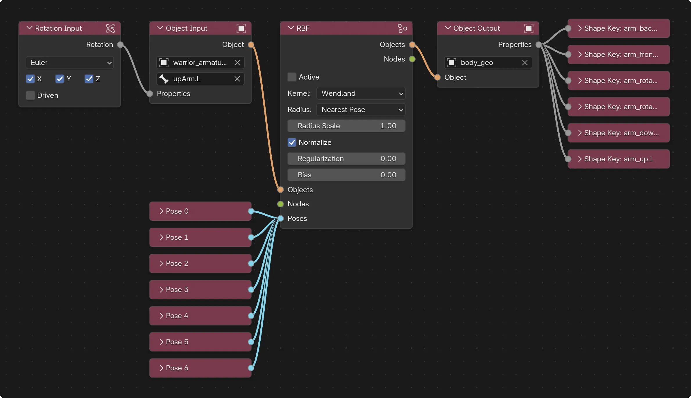
6.5 Activating the Solver
- Once poses are defined, click Activate in the Sidebar.
- The RBF node computes interpolation weights and updates the background color:
- Green: The solver is active.
- Red: Error (see Troubleshooting )
6.6 Resetting the Setup
- To remove driver links and deactivate the solver, click Reset.
7. Defining Input Properties
Input properties determine what drives the RBF interpolation. They consist of an Object Input node to select the source, plus one or more Property Input nodes to choose specific properties.
7.1 Input Object Node
Object/Bone Name
Enter the name of the driver object or bone.
Only the name of the driver object or bone is stored, not a direct reference to the object’s data block. Storing a pointer would interfere with linking the RBF setup into another scene. Because only the name is stored, it does not reflect any name changes that might occur after assigning the object to the node.
Properties Socket
Receives connections from
Property Input
nodes.
7.2 Property Input Nodes
Add via Shift + A → Input or from the menu choose Add → Input.
Available property nodes are:
Location
The location of the object. Use
Driven
to include the evaluated location based on constraints and drivers.
Rotation
The rotation of the object. Use
Driven
to include the evaluated rotation based on constraints and drivers.
Scale
The scale of the object. Use
Driven
to include the evaluated scale based on constraints and drivers.
Property
A float-based property of the object which can be used as a driving value.
Custom
A custom property of the object which can be used as a driving value.
- Auto: Select the property from the list.
- Manual: Select the property by name in case it’s not included in the list.
Switching between Auto and Manual copies the name of the property from one to the other. If the manually entered name doesn’t exist on the object, it is skipped.
Shape Key
A shape key of the object.
- Auto: Select the shape key from the list.
- Manual: Select the shape key by name in case it’s not included in the list.
Switching between Auto and Manual copies the name of the shape key from one to the other. If the manually entered name doesn’t exist as a shake key, it is skipped.
When set to Auto, the shape key in the list depends on its actual position in the shape key list on the object. If the shape keys are re-ordered, a different shape key will be referenced in the node. To prevent this behavior, first select the shape key in the list while set to Auto, and then switch to Manual. This sets the shape key to be referenced by its name, not by its position in the shape key list.
Modifier
A modifier of the object. With the modifier selected a second drop-down menu displays available properties.
Node
This node is automatically created when selecting a node in the currently open Shader or Geometry Nodes editor and pressing the
Link Input Node
button on the Sidebar.
- Parent Type: The data-block type of the node’s parent; either Node Group or Material.
- Parent: The name of the node’s parent.
- Node: The name of the node in the material or node group.
- Plug: The actual internal identifier of the property selected in the drop-down menu below.
- Property: The name of the property to be used as the driver.
Steps to add and connect:
- Shift + A → Input → [Property Type] or from the menu choose Add → Input → [Property Type].
- Connect the property node’s output to the Properties socket of the Object Input node.
- Configure available properties on the Property node.
- For shader- or Geometry Node-driver outputs, associate the target node via Link Output node in the RBF Nodes editor and select the diving property on the node.
8. Defining Output Properties
Output properties specify targets that will be driven by the RBF solver. The setup procedure is mirroring the input setup. After activating the RBF they feed into the scene via driver expressions.
Every output property node includes an Output Range setting, which controls how the output handles values between and beyond the poses:
- Bounded keeps the result within the pose values, like a shape key that shouldn’t go past 0 and 1.
- Unbounded lets the result travel further out than the poses, useful for a location or another value that needs to keep going.
- Automatic picks Bounded or Unbounded based on the property type. This is the default.
8.1 Output Object Node
Object/Bone Name
Enter the name of the driven object or bone.
Only the name of the driver object or bone is stored, not a direct reference to the object’s data block. Storing a pointer would interfere with linking the RBF setup into another scene. Because only the name is stored, it does not reflect any name changes that might occur after assigning the object to the node.
Properties Socket
Outputs connections to the
Property Output
nodes.
8.2 Property Output Nodes
Add via Shift + A → Output or from the menu choose Add → Output.
Available property nodes are:
Location
The location of the object. Use
Driven
to include the evaluated location based on constraints and drivers.
Rotation
The rotation of the object. Use
Driven
to include the evaluated rotation based on constraints and drivers.
Scale
The scale of the object. Use
Driven
to include the evaluated scale based on constraints and drivers.
Property
A float-based property of the object.
Custom
A custom property of the object which can be driven.
- Auto: Select the property from the list.
- Manual: Select the property by name in case it’s not included in the list.
Switching between Auto and Manual copies the name of the property from one to the other. If the manually entered name doesn’t exist on the object, it is skipped.
Shape Key
A shape key of the object.
- Auto: Select the shape key from the list.
- Manual: Select the shape key by name in case it’s not included in the list.
Switching between Auto and Manual copies the name of the shape key from one to the other. If the manually entered name doesn’t exist as a shake key, it is skipped.
When set to Auto, the shape key in the list depends on its actual position in the shape key list on the object. If the shape keys are re-ordered, a different shape key will be referenced in the node. To prevent this behavior, first select the shape key in the list while set to Auto, and then switch to Manual. This sets the shape key to be referenced by its name, not by its position in the shape key list.
Modifier
A modifier of the object. With the modifier selected a second drop-down menu displays available properties.
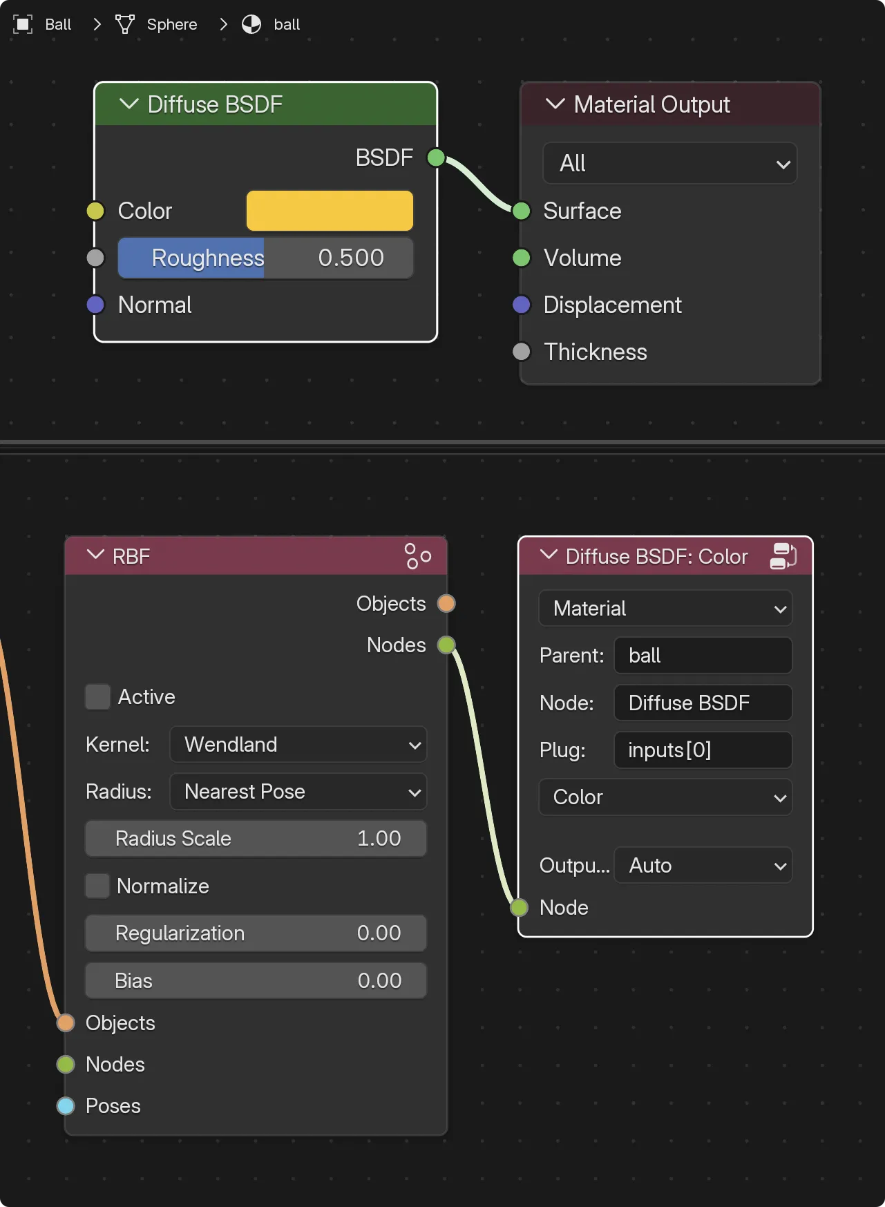
Node
This node is automatically created when selecting a node in the currently open Shader or Geometry Nodes editor and pressing the
Link Output Node
button on the Sidebar.
- Parent Type: The data-block type of the node’s parent; either Node Group or Material.
- Parent: The name of the node’s parent.
- Node: The name of the node in the material or node group.
- Plug: The actual internal identifier of the property selected in the drop-down menu below.
- Property: The name of the property to be driven.
Steps to add and connect:
- Shift + A → Output → [Property Type] or from the menu choose Add → Output → [Property Type].
- Connect the Output Object node’s Properties socket to the property node’s property socket.
- For shader- or Geometry Node-driven outputs, associate the target node via Link Output node in the RBF Nodes editor and select the driven property on the node.
9. Creating and Managing Poses
Poses define sample states for both driver and driven values, forming the basis for interpolation.
In general, it’s important to have a minimum set of poses for the RBF to interpolate between. The first pose should always be the rest pose, where all driving and driven values are at their default. Since RBFs are mostly used to blend between a set of extreme property values or poses around a central default pose, it is expected to have a rest pose and at least two poses to evaluate between. Even if it were possible to have only two poses, the rest and a target pose, this would invalidate the need for an RBF solver. Usually, it’s best to use at least three to five poses to achieve smooth interpolation over a range of motion.
9.1 Adding a Pose
- Set the properties used as input drivers to assume the pose.
- Set the properties used as driven outputs to assume the pose.
- Click Add Pose in the Sidebar.
- A Pose node appears and connects to the RBF node’s Pose socket.
The Pose node stores the current values of all connected inputs/outputs.
Every pose of a setup has to hold the same properties. Adding an input or output after the first pose exists is therefore refused, until the existing poses have been updated to include the new set of properties. See Changing Inputs and Outputs Later.
9.2 Editing a Pose
- Click Edit on the Pose node.
- Modify the values in the scene.
- Click Edit again to save the changes.
Only one pose per RBF node can be edited at a time. When another pose is already in edit mode a message appears and the button stays off.
9.3 Recalling a Pose
Select a Pose node and click Recall to apply its stored values to the scene.
Recalling a pose by applying the stored values to the related objects or data-blocks in the scene does only work if the properties are directly accessible. If properties are driven or have underlying constraints it’s not possible to recall the pose properly.
9.4 Deleting a Pose
Select the Pose node and delete it.
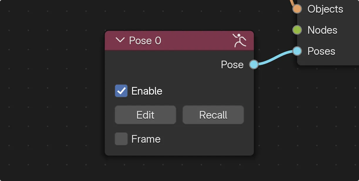
9.5 Disabling a Pose
When a pose is enabled (the default), it contributes to the RBF solution like any other. When disabled, the pose is removed from the calculation entirely; the solver behaves as if it were never created, and the remaining poses are re-solved without it. Toggling Enable triggers an automatic re-solve, so changes take effect immediately.
Use it to test how a setup behaves with a pose taken out, or to keep an in-progress pose in the tree without having it affect the result. Note that removing a pose this way changes how the neighbouring poses interpolate, since the solution is rebuilt over the remaining set.
9.6 Pose Frames
Setting up poses can be an elaborate task, as it requires constantly adjusting all driving and driven properties. Especially when working with a combination of armatures, bones, other objects, and their related properties. A lot of back and forth and switching between modes is essential. As a result, it’s easy to overlook a setting, which then makes it necessary to go back and edit the pose or even start over. Also, editing a pose always requires rebuilding all the values for the particular pose.
As a helper function, it is possible to recall a pose , however, this is limited if underlying constraints or drivers are involved.
Therefore, it is recommended to set up a Range of Motion (ROM) animation prior to creating the first pose. This animation is used to go through all extreme values of the participating elements and objects which are important for the overall articulation. The advantage is twofold: it not only makes it much easier to see everything in action, but these extremes can also be used for defining the poses.
With this ROM animation in place, everything is displaying the actual result of keyframed animation and rigging dependencies, and it’s much easier to use this as the base for defining and editing poses.
To support this workflow, the current frame is saved along with the pose to make recalling a pose more complete in terms of constraints and other drivers.
If a pose has a frame stored, a Frame checkbox will display on the Pose node.
Poses which have been created in legacy RBF Nodes setups have no frame property set, and the checkbox will be hidden.
With the pose frame present, there are two options to recall a pose:
Frame turned off
The pose will be recalled by applying the stored values of the pose, independent of the current frame. If the driven object is constrained or driven, the visual result will not match the actual pose.
Frame turned on
The animation will jump to the stored pose frame before the values of the pose are applied. This ensures that the visual pose reflects the actual state the pose was created in. Of course, this only works if the
Range Of Motion
animation is still in place, which has been used to set up the poses.
9.7 Changing Inputs and Outputs Later
When creating a setup it is common that the need for additional inputs or outputs changes while poses have already been created.
Because all poses need to store the same set of properties, as defined by the inputs and outputs, it is not possible to add a new pose with Add Pose after new input or output properties have been added. This action is refused because it would lead to the new pose storing more properties than are contained in the other poses.
However, it is possible to update all existing poses to reflect the changed setup with its additional inputs or outputs and therefore contain the increased number of properties.
Update Poses reads the current inputs and outputs and adds every missing property to the existing poses, which have been created with a different property count.
9.7.1 Adding an Input or Output
- Create and link the new input or output node, the same way as for a new setup.
- Click Update Poses in the Sidebar.
- Continue with Add Pose as usual.
- Activate the solver again, so that the new properties are included in the computation.
If the solver is active while a new property is enabled, the node reports that the number of pose and driven properties doesn't match and switches off. This is expected. Enable the remaining properties of the new node and continue with Update Poses.
The value written to the existing poses for a newly added property is the value it has when Update Poses is executed. A property which was not part of the setup before can be assumed to be at its rest value for all existing poses at the time when _Update Poses_ is performed. This property is only changed before the new pose is created and therefore contributes a different value to the new pose.
It is important to note that Update Poses should be performed directly after creating new inputs or outputs and before adjusting the newly added properties. If the new input or output is posed first, the current values are written to the existing poses, and creating a new pose doesn't store any different values.
A shape key output is the one exception which needs no extra step. It can be added at any time and Add Pose accepts it directly, filling in a value of 0.0 for the existing poses.
9.7.2 Removing an Input or Output
Removing is not supported.
A stored pose keeps its values under the name of the property they belong to, and that is how Update Poses knows which stored value goes with which input or output. Where every property of an object has a name of its own, such as the three location axes of a bone, a name is enough to tell them apart. A node socket which contains several channels reports the same name for all of them. For example, a colour connects as four properties, separated only by their position in the set.
If one of these is removed, the following ones move up a position, which results in a different order than before, without any indication of which one has been removed. The changed value assignments then lead to an incorrect evaluation and a visibly wrong result.
Therefore, an input or output cannot simply be removed without disrupting the current setup. When Update Poses is used on such a setup, the action is refused and the missing properties are listed in the console output. If such an error occurs, this information can help to identify the missing properties and relink them.
If an input or output needs to be removed from a setup which already contains poses, the best solution is to delete the poses and create them again. A setup can always be expanded by adding properties, but removing one or more requires rebuilding it.
10. RBF Settings
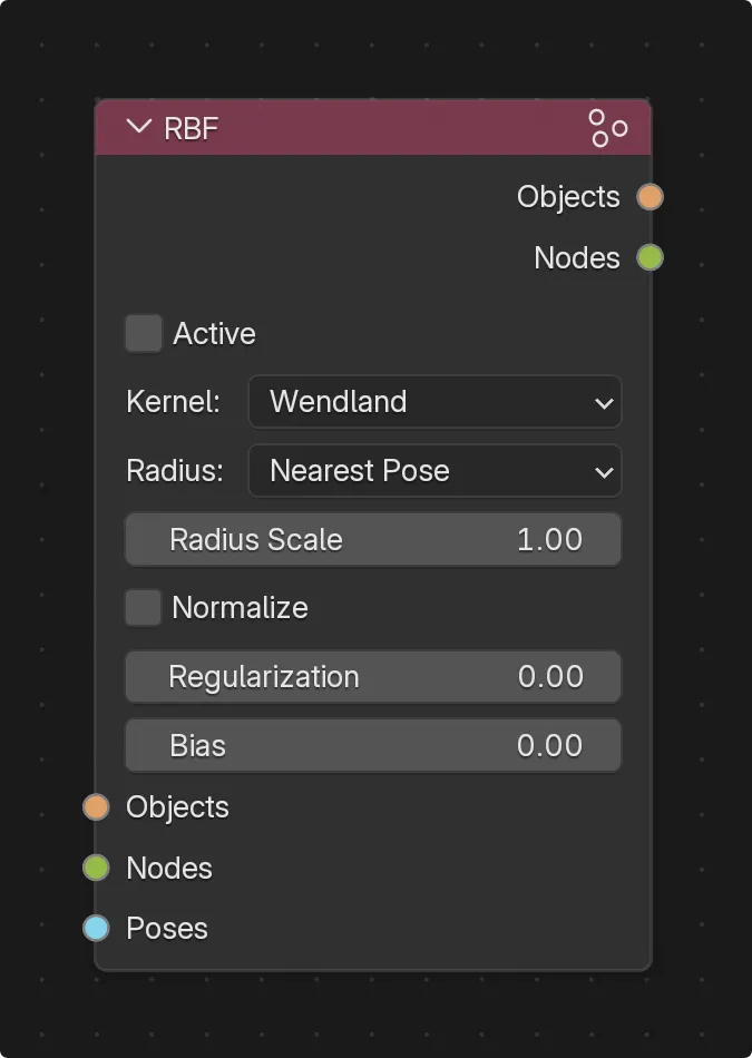
10.1 Kernel
The Kernel determines the mathematical function used by the solver to calculate how much each pose contributes based on its distance from the current input. In simple terms, it’s the shape of the influence falloff curve around each pose.
Different kernels have different blending behaviors:
Wendland
Falls off smoothly and reaches zero beyond its radius, so poses that are far apart have no effect on each other at all. This makes it the most predictable kernel, and it’s the default for new setups.
Gaussian
Smooth and localised, this kernel falls off quickly as the input moves away from a pose, though it never quite reaches zero. It produces clean, natural blends.
Linear
Influence drops off in a straight line. This is simpler but may result in harsher transitions or artifacts.
Inverse Multi-Quadratic Biharmonic
Smooth, long-range influence that gradually fades as distance increases. Less aggressive than Gaussian, with broader coverage. It may be used to have influence over a wide range without a sharp drop-off.
Choosing the right kernel depends on the kind of deformation or behavior aimed for. Wendland is a safe default, but experimenting with other kernels can produce useful variations in blending behavior.
10.2 Radius
The Radius controls how the solver determines the influence radius (also called kernel width) for each pose. This affects how far a pose’s effect reaches across the input space, which in turn shapes how blending between poses occurs.
A small radius means that poses will only affect the result when the input is very close to them, creating sharp transitions. A larger radius allows poses to influence a broader area, resulting in smoother blends and overlap between poses.
Nearest Pose
Automatically gives every pose its own radius, based on the distance to its closest neighbouring pose. This is what keeps an uneven spread of poses just as stable as an evenly spaced one, since what matters for blending is how close poses sit to each other, not how far the whole set of poses reaches.
Custom
Allows the radius to be set manually as a single, fixed value shared by every pose. This ignores how the poses are actually spaced, so it’s best kept for situations where full, direct control over the falloff range is required rather than used as a general default.
When Nearest Pose is selected, a Radius Scale value takes the place of the manual radius. It widens or narrows every pose’s radius relative to its closest neighbour. A value of 1.0 is stable for any number of poses; higher values blend more broadly, at the cost of more overshoot between poses.
10.3 Normalize
This toggle scales the input values before the solver measures how far apart the poses are.
The inputs are scaled in groups, so channels which belong together, such as location or rotation, keep their proportions. When active, every group is divided by its typical size across all poses. For location it's the average distance from zero, for rotation, how far it is turned away from zero rotation. This lets every group contribute on a comparable scale to the distance between poses. Without it, one input might dominate the others purely because of its numeric scale, for example rotation in radians vs. distance in scene units.
Every driving object or bone has its own groups, so two bones form two groups even when both only use their rotation. With a single group and the Nearest Pose radius the toggle has no effect, because the distances and the radii are scaled together. It becomes relevant as soon as more than one group is involved, or when a Custom radius is used.
In some cases, particularly when intentionally relying on differences in scale between inputs, it may be preferable to leave it disabled, so that the solver works with the original, unmodified input values.
10.4 Regularization
When solving the pose‑weight matrix, very similar poses can sometimes make the system unstable, leading to errors or unpredictable results. The regularization parameter (also known as Tikhonov epsilon) helps guard against these issues. It can stabilise the solver and penalises overly large weights, trading a bit of perfect accuracy for much greater reliability.
The range can be set between 0 and 10, where 0 disables regularization entirely. A value of 1 is barely noticeable. A value of 5 is a commonly used default, which is still small, but effective. A value of 10 applies strong regularization and starts to noticeably flatten the poses.
10.5 Bias
The Bias property adjusts how sharply or softly the influence of each pose fades in and out during blending.
This setting reshapes the weight curve used by the solver:
- A positive bias sharpens the falloff, making poses activate more strongly when close to the input and fade out quickly when moving away. This is useful when needing crisp, punchy transitions.
- A negative bias softens the transition, allowing poses to remain active over a broader range. This can help create smoother or more forgiving blends between poses.
- A bias of 0 disables the effect and uses the raw solver output without reshaping.
The value ranges from -3 to 3.
Example: If a pose doesn’t hold its influence long enough as the input moves past it, using a slightly negative bias can help to extend its effect.
The bias reshapes each pose’s own weight before it contributes to the output, so it does not change which poses are active, only how strongly each one contributes. A Bounded Output Range still keeps the result within the pose values regardless of the bias used.
10.6 Condition Number
Once the RBF is active, the node shows a Condition value below its other settings. This is a read-out of how sensitive the solve is to small changes in the poses. A small value is healthy. A large value, shown in red, means two or more poses sit too close together and the result may not be reliable.
If the value turns red, moving the closest poses further apart, or removing one of them, is usually the fix. See Troubleshooting.
10.7 Estimated Radius Scale
This is measured from the pose data alone whenever the solver is solved, and suggests a Radius Scale value as a starting point for fine-tuning the interpolation. It checks how far other outputs rise between each pose and its closest neighbour, and returns the widest value which keeps them below 5 % of their range.
11. RBF Activation and Evaluation
Upon activation the system computes the RBF interpolation weights based on defined poses and applies driver expressions to outputs for real-time evaluation.
Processing the distance matrix from the given pose values and solving the required equations can be computationally expensive, particularly with large datasets or complex rigs evaluated on a per-frame basis. To keep playback efficient, RBF Nodes performs the heavier computations, such as pose comparisons and kernel weighting, when the solver is activated. At runtime, only the minimal necessary interpolation is calculated, ensuring performance remains smooth even with multiple or complex setups.
This design reflects a common characteristic of Radial Basis Function solvers: most of the computational cost lies in the setup phase, while evaluation is relatively lightweight. However, the cost still scales with the number of input drivers, output targets, and poses in the system. Keeping the pose count efficient and avoiding unnecessary redundancy in inputs or outputs can help maintain optimal performance.
In summary:
- Heavy computations (e.g. distance matrix, solver weights) occur when the RBF is activated.
- Light computations (e.g. interpolation) occur during playback.
- To maintain performance, limit excessive pose counts and keep the input/output setup lean.
- Consider disabling the solver when not in use.
This structure allows RBF Nodes to offer responsive, interactive rigs without compromising runtime speed.
11.1 Activating RBF
- Ensure at least three Pose nodes are connected to the RBF node.
- Click Activate in the Sidebar.
- The RBF node performs internal calculations:
- Builds the distance matrix from input poses
- Solves for weight coefficients
- Generates driver expressions for each output property
- Status indication:
- Green Background: Activation succeeded
- Red Background: Activation failed (see Troubleshooting )
11.2 Runtime Evaluation
- On frame change or input value update, Blender evaluates driver expressions, applying interpolated values to outputs with minimal overhead.
11.3 Resetting RBF
Click Reset in the Sidebar to remove driver expressions.
11.4 Adjusting Solver Properties
Even after the RBF is activated, its core properties can still be adjusted, such as Kernel, Radius, Bias, or Normalization. These changes directly affect how the solver calculates weights, so modifying them will automatically reinitialise the RBF in the background to reflect the updated configuration.
This allows to fine-tune the solver’s behavior without needing to deactivate or recreate the setup.
However, once the RBF is active, structural edits are have no effect:
- Adding or removing input or output properties.
- Creating new pose nodes.
- Input/output properties are locked.
This ensures the solver operates on a stable structure but still provides flexibility to adjust the behavior of the interpolation.
12. Scene Linking and Library Overrides
RBF setups can be linked across multiple Blender scenes as part of a rig for modular workflows. This enables maintaining a rig in one scene and using it in another.
After linking it is important to create a Library Override for the rig and all related objects. Without overrides, the solver cannot access linked data, and the setup will fail.
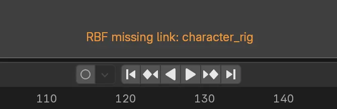
An on-screen message informs about missing data in the RBF setup.
This is an indicator that the linked data hasn’t received a library override yet or that the library override has indeed caused some data to be duplicated.
In this case it’s necessary to cross-reference the names assigned to the Object Input and Output nodes with the object names of the linked data.
Name-Based References: Object Input/Output nodes reference objects by name. Renaming linked objects requires updating the node’s name field.
13. Constraint and Driver Support
RBF Nodes supports transformations from constraints and drivers, allowing for more flexible setups and eliminating the need for additional helper bones or rigging workarounds.
To include indirect transformations, such as those coming from constraints or drivers
- turn on Driven on any transformation Input node or Output node
Enabling this option ensures that Blender evaluates all dependencies correctly, including constraint-influenced rotations or positions, rather than just using raw channel values.
This option is not enabled by default, as it is not essential in most cases. Enabling it introduces additional matrix multiplications, which can lead to less precise results, particularly for rotations, due to floating-point precision errors. It should therefore only be used when necessary and left off if the transformation can be accessed directly.
If jittery motion is still visible, even after adjusting the base RBF properties Kernel and Radius it might be necessary to activate Smoothing, even though it might introduce some delay in responsiveness. See Rotation Smoothing
14. Rotation Smoothing
When working with constrained or driven rotations, Blender internally performs matrix calculations using floating point math. While these calculations are very precise, even minor rounding differences can cause visible artifacts when used as input for RBF solvers. This is because RBF interpolation is highly sensitive to small changes in rotation, often interpreting even minor noise as meaningful variation. The result can appear as jittery or unstable motion in the output.
In most cases, this issue can be mitigated by adjusting the Kernel and Radius settings of the RBF node, which control how broadly and smoothly influence is spread between samples. A slightly wider radius or softer kernel function can help smooth out minor inconsistencies.
For additional control, especially when working with driven objects, bones or quaternion-based input, the Smoothing option can be enabled on the node.
Smoothing works by comparing the current rotation to the previous frame and blending them together, effectively filtering out micro-jitter or subtle numerical noise. This is particularly useful in setups where constraint evaluation introduces tiny but frequent changes that would otherwise cause visual instability. While smoothing helps create a more stable and natural result, it’s important to note that it introduces a small time-based dependency, meaning extremely fast changes in rotation may feel slightly delayed depending on the blend strength.
By carefully balancing the RBF solver settings with the smoothing option, responsive yet stable interpolation can be achieved even in complex driven or constrained rigs.
14.1 Smoothing Properties
When enabling Smoothing on a transformation node, a few properties become available to fine-tune how it behaves. These settings help reduce jitter or instability, especially when using constraint-driven or quaternion-based input.
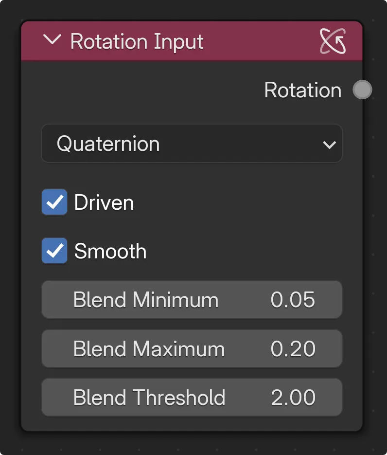
Blend Minimum
- The minimum amount of smoothing applied when rotations change only slightly.
- It serves as the baseline: even when there’s very little motion, this value keeps things gently smoothed.
- A value around 0.05-0.2 is typically subtle and effective.
Blend Maximum
- The maximum amount of smoothing, used when rotation changes are extremely small, often just noise.
- Higher values apply stronger filtering but may introduce a slight delay in responsiveness.
- Lower values feel more immediate but may let more jitter through.
- A range of 0.1–0.3 serves as a starting point, with adjustments made depending on the desired stability or responsiveness of the motion.
Blend Threshold
- The rotation difference (in degrees) at which smoothing is turned off completely.
- If the rotation changes significantly between frames (e.g. from fast movement or user input), smoothing is skipped to avoid unwanted lag.
- Values around 2°-5° are a good starting point.
14.2 Smoothing Practice
Smoothing compares the current frame’s rotation with the previous one. If the difference is small, it blends the two together for a smoother result. If the difference is large (above the threshold), it assumes the change is intentional and applies no smoothing to keep the motion responsive. This allows the animation to feel stable when idle, but still sharp when moving.
15. Preferences
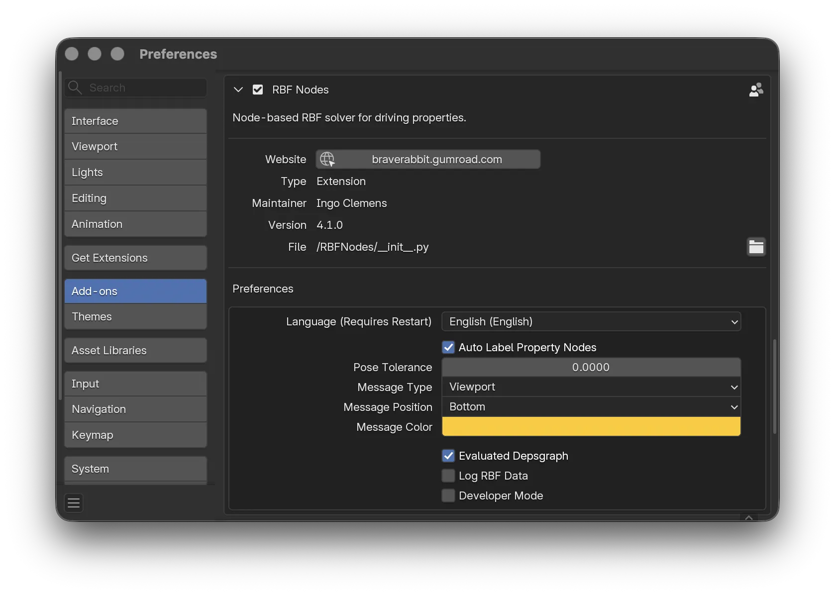
15.1 Auto Label Property Nodes
With this option enabled the label of property and shape key nodes will be automatically set to reflect the chosen or entered property name. This makes the node tree easier to read when the nodes are minimised.
15.2 Pose Tolerance
Sets the precision threshold used to detect whether a newly created pose is effectively identical to an existing one. If all values fall within the specified tolerance, the pose is considered a duplicate and will be rejected.
This prevents redundant poses that could lead to decomposition issues or unstable solver behavior. Increase the value slightly if precision errors are causing near-identical poses to be treated as unique.
15.3 Message
These properties define the position and style of the warning message shown after linking a scene that contains an RBF setup. The message alerts that the RBF cannot be evaluated or that required library overrides are missing.
15.4 Evaluated Depsgraph
When enabled, the evaluated object data is used for computation. This is necessary for calculating constrained or driven transformations and for evaluating linked RBF setups. Primarily intended for debugging purposes.
15.5 Log RBF Data
Writes the RBF data to the command output during pose creation and RBF activation. Primarily intended for debugging purposes.
15.6 Developer Mode
Enables additional properties on the output nodes for debugging purposes.
15.7 Config File
In addition to Blender’s standard preferences, all RBF Nodes settings are stored in a config.json file located at the top level of the extension. This ensures that extension-specific preferences remain intact even if Blender’s preferences are reset.
16. Advanced Settings
This chapter covers the advanced controls available in the Advanced sub-panel of the RBF Nodes Sidebar.
16.1 Edit Pose Properties
When working with pose nodes, each one stores references to Blender objects and properties as plain text. These references are used to define both the driving inputs (which trigger a pose) and the driven outputs (which respond to a pose). However, if an object or property is renamed later in Blender, the references stored in the poses will not update automatically.
To help manage this, the Sidebar includes two tools that allow to find and replace object and property name references across all poses.
These tools don’t change the actual names of objects or properties, they only update the string references stored in the poses. This makes it a safe and convenient way to keep the setup working even after changes to names elsewhere in the file.
To avoid unexpected behavior, double-check the console output (using the View Pose Data button) before and after running a rename operation. This can help to verify that the correct references were updated.
Rename Driver or Driven References
The operators update the property paths used as inputs or outputs to the poses — in other words, the values that activate or effect a pose.
- Search: Enter the part of the property path to find.
- Replace: Enter the text to replace with.
- Driver or Driven: Apply the change to all driver or driven references in every pose.
Use this when the name of a control property or object that acts as an input or output to the solver has been changed.
16.2 View Pose Data
This button prints out all the data linked to the currently selected pose node. It will display two blocks of information in the system console:
Driving Values
These are the input values that define how the pose is activated. They’re shown in Blender’s full data path format, such as:
bpy.data.objects["Cube"].location[2] = 12.5
This shows which object and property are being used, and what value is stored.
Driven Outputs
These are the values the pose affects when it becomes active. This makes it clearly see which objects and properties are being controlled.
This tool is helpful for several reasons:
- It gives a clear, readable list of everything that makes up a pose.
- It makes it easy to double-check whether the right properties are being referenced.
- If something isn’t working as expected, this output can be used to spot outdated or broken links. For example, if a property was renamed after setting up the pose, the reference stored in the pose won’t update automatically (just like Blender drivers).
By reviewing this output, it’s possible to identify incorrect or missing property paths and to fix them before they cause errors during animation or solver setup.
16.3 View RBF Data
This button allows to inspect the internal pose matrix used by the RBF solver. Each time a pose is added to the system, its values are stored as part of a matrix that the solver uses to calculate smooth transitions between poses.
If something goes wrong during the setup, like adding duplicate poses or entering invalid values, the solver might fail to complete its calculation. In such cases, this tool can help to understand what’s going wrong by giving a clear, detailed view of the raw pose data.
When selecting RBF in the View Data section, the full contents of the pose matrix will be displayed in the system console. Each row of the matrix corresponds to one pose, and each column represents a value (like a control or driver) that defines the shape or state of that pose.
By examining this matrix, it’s possible to:
- check for duplicate poses (rows that look the same)
- spot any unusual values (such as missing data or extreme numbers)
- better understand how the solver interprets the pose data
This tool is especially useful if an error is encountered during the solver’s setup phase. If an error message informs that the process failed at a specific pose index, the matrix output will help to find the problem directly.
16.4 Export and Import
A setup can be written out as a json file and rebuilt from one. This is different from View RBF Data, as it describes the RBF node tree itself with all the contained data, so that it can be rebuilt.
There are two reasons to use a setup file:
1. Manual data editing and correction
If it is necessary to edit one or more poses, it can be easier to edit the data in a text editor than to use Edit on the Pose node, which can easily lead to incorrect values being stored. The same applies to renaming properties throughout, or removing values. The file is plain json and can be edited with anything, then imported back.
2. Repairing a setup
If a node tree has been damaged by rearranging or deleting nodes, the last exported file acts as a backup. Even when the file itself needs to be edited by hand, it is a way of working on the data outside the editor.
16.4.1 Setup Export
Writes the node tree currently shown in the editor. The file is stored in an RBFNodes folder beside the saved scene, or in the system's temporary folder when the scene has not been saved yet. It is named after the node tree with a sequence number. The setup file only contains the node tree and pose data. That is all that's needed to rebuild the solver setup.
16.4.2 Setup Import
Opens the file browser at that same folder, so the right version can be picked from the ones which are there.
The file stores which node tree it was written from, and that tree is the one it is rebuilt into. If the scene has no tree of that name, one is created instead, which is what makes it possible to import a setup into another scene.
The solver is left switched off afterwards. Press Activate to solve it and build the drivers again.
Objects referenced in the file which are not in the scene do not stop the import. The tree is built with the names it was given and the ones which could not be found are listed in the console.
17. Troubleshooting
Solver Activation Error
When activated, the
RBF
node displays a red background along with an error message. This usually indicates problematic data in one or more
Pose
nodes, providing insufficient or inconsistent input for the solver to process.
Although several checks are performed when creating a pose to ensure alignment with existing pose data, it is still possible for invalid data to pass through and cause the solver to fail.
Common causes for activation errors include:
- Too few poses
- Similar or duplicate poses
- Poses containing a different number of driver or driven values
Value-related issues can typically be identified by inspecting the Pose or RBF data, or by checking the Condition Number shown on the RBF node once it’s active.
Too few poses
At least three poses are required for meaningful interpolation: a rest pose and two extremes. A setup with only two poses eliminates the need for an RBF solver. Generally, at least three to five well-defined poses are recommended to achieve smooth interpolation across the full range of motion.
Too many poses
While there is no strict upper limit, having too many poorly distributed poses can introduce problems. Most issues arise when poses are clustered too closely or are nearly identical. A well-balanced distribution is essential for stable results.
Driver creates no output
If an object or bone is constrained, its transformation may not be directly available, as Blender computes it internally. By default, only direct property values are evaluated.
To process transformations affected by constraints or drivers, enable the
Driven
option on the corresponding transform property node.
Note: Enabling the Driven option introduces additional matrix computations, which may reduce precision, especially for rotations, and lead to instability.
Jitter
If visible jitter remains even after adjusting the core
RBF
properties (
Kernel
and
Radius
), enabling
Smoothing
may help stabilise the output. However, this can introduce slight latency in responsiveness. See
Rotation Smoothing
Disclaimer
This documentation reflects the current state of RBF Nodes for Blender. Functionality and features may evolve in future releases.
Copyright (C) 2022-2026, Ingo Clemens, brave rabbit,
www.braverabbit.com
GNU GENERAL PUBLIC LICENSE Version 3